← Back to list


PatchCore
Anomaly Detection
Anomaly Detection (AD) is widely used across various fields. In security, it can be applied to detect external intrusions, while in healthcare, it can be used to distinguish between healthy individuals and patients.
In this post, I would like to introduce PatchCore, one of the most representative models among image-based AD techniques used in the manufacturing sector. Published in 2022, this paper has long served as a benchmark baseline model in image-based anomaly detection research and remains a cornerstone architecture in the field.
In industrial settings, 2D image-based Anomaly Detection (AD) is primarily used to detect surface defects on products. Generally, computer vision classification and segmentation models can evaluate product quality (normal vs. defective) and localize defect areas, but because both are supervised learning methods, data labeling is strictly required. Deep learning-based supervised models typically require at least 1,000 training samples to build a model with reliable performance.
However, in real-world manufacturing environments, defective products are rarely produced, making it time-consuming to gather large volumes of defective data. Conversely, normal product data is easily obtained. AD techniques are specifically suited for such scenarios where the goal is to detect defects despite defective data being extremely scarce.
PatchCore
PatchCore is one of the representative AD models that performs anomaly detection using a memory bank mechanism. The memory bank approach falls under embedding-based methods, alongside reconstruction-based methods and synthesis-based methods.
PatchCore is an enhanced model that addresses the limitations of PaDiM; it achieves faster inference speeds and improves anomaly detection performance by incorporating context from neighboring patches, whereas PaDiM relies solely on isolated individual patches. (I will skip the detailed explanation of PaDiM for now.)
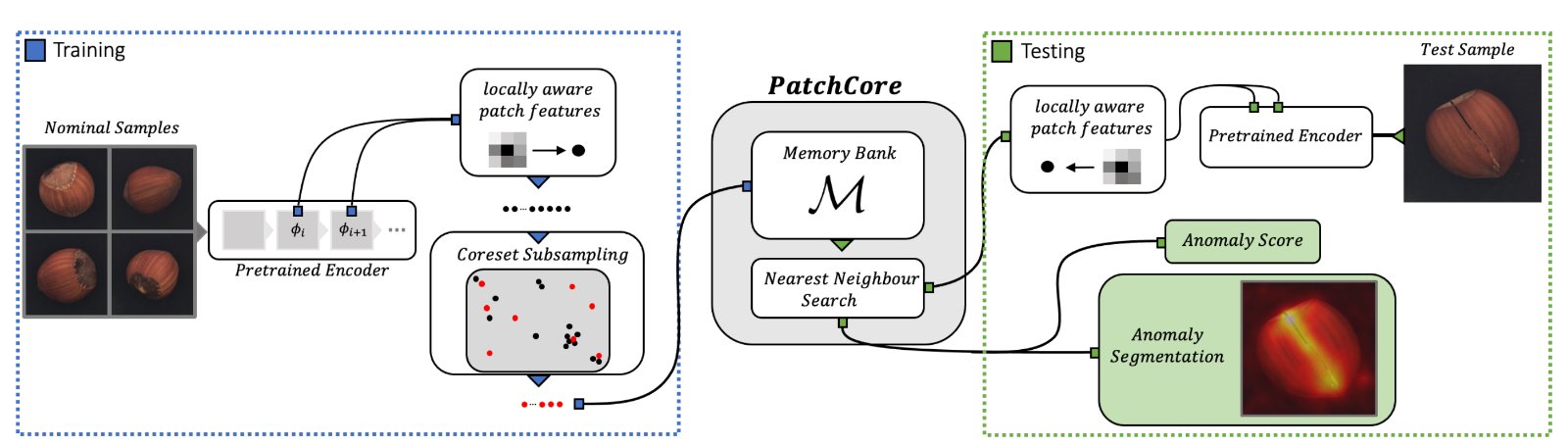
The overall process of PatchCore is illustrated in the figure below:
. . .
[Training]
1. Feature extraction is performed by passing normal sample image data through a CNN-based model such as Wide-ResNet.
- The features are extracted from intermediate layers of the model rather than the final layers.
- Extracting features from deeper (later) layers causes the features to be heavily influenced by the dataset on which the model was pre-trained, which can incorporate characteristics of the pre-training dataset rather than preserving the specific properties of the target image we intend to extract.
- On the other hand, using early layers fails to extract meaningful feature representations because the layer representations are too low-level/undeveloped.
2. The extracted feature patches are aggregated with neighboring patches to form a single representative patch.
- In the paper, Adaptive_average_pool2d is used to aggregate contextual information from neighboring patches.
- There are two aggregation approaches: aggregating features extracted from a single layer, and the Multi-Hierarchy approach, which aggregates features extracted across two layers.
- Multi-Hierarchy Aggregation individually aggregates features from two different layers, aligns their feature shapes, concatenates them, and then aggregates them once more to match the target dimension.
- According to the study, using multi-layer feature representations yields better performance than relying on a single layer.
- This is because combining intermediate-level layers with higher-level layers captures a richer set of feature representations.
3. Coreset Subsampling
- Only important patches are selected from the aggregated feature patches obtained in Step 2.
- Prior to selection, high-dimensional feature patches are projected into a lower-dimensional space to reduce computational complexity.
- Random projection based on the Johnson-Lindenstrauss lemma is employed as the low-dimensional projection method.
- According to the Johnson-Lindenstrauss lemma, when points in a high-dimensional space are projected into a suitable lower-dimensional space, pairwise distances are approximately preserved.
- After performing the low-dimensional projection, the coreset Mc that satisfies the following condition is identified:
4. Build the memory bank with the coreset Mc.
- Example: The process of finding Mc after projecting features into a low-dimensional space in Step 3 during training
1. First Iteration- The first index (index 2) is chosen randomly. In the next iteration, the 4th patch—which has the maximum distance of 16 (in red)—is selected for comparison.
- Euclidean distance represents similarity: a smaller distance indicates higher similarity, whereas a larger distance indicates lower similarity.
- The maximum distance value of 16 implies that the 2nd patch and the 4th patch represent significantly different data patterns.
→ It is highly likely to be a unique data point.
→ Its features are distinctive/prominent.
→ It is highly likely to be a core patch that acts as a key representative among numerous patches.
2. Second iteration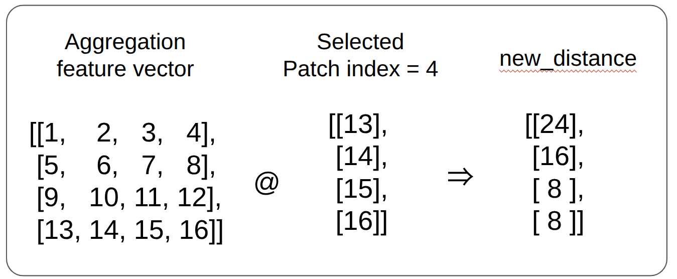
- Calculating Euclidean distances between the 4th patch and other patches
- Select the minimum distance values across existing coreset patches, and among those, pick the 1st patch that exhibits the maximum distance value (in red).
- Selecting the minimum values means finding the closest/most similar representative patch for each candidate point. Choosing the maximum among these minimum values implies that even after pairing each candidate with its closest neighbor in the coreset, this candidate remains the most distant from the current coreset.
- Selecting the patch with the largest Euclidean distance = selecting the most distinctive/unique patch.
- Since the memory bank should store unique features of the product rather than ordinary/redundant background data, saving these distinctive patches in the memory bank makes it easier to distinguish differences when compared against anomalous data later.
3. Final Memory Bank
- Only the patches corresponding to the selected indices are stored in the memory bank.
=> selected_index = Coreset Subsample index = [2,4,1]
[Testing]
1. Perform Steps 1 and 2 of the Training process on the test image in the exact same manner.
2. Calculate the Anomaly Score (AS) using the test image's feature patches and the memory bank.
- The maximum patch-level AS is considered the representative Anomaly Score for the entire image.
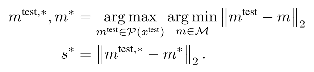
- Anomaly Score Formula:
- Rather than directly using the Euclidean distance between a test patch and the memory bank as the anomaly score, a weight calculated via softmax is applied to determine the final anomaly score.
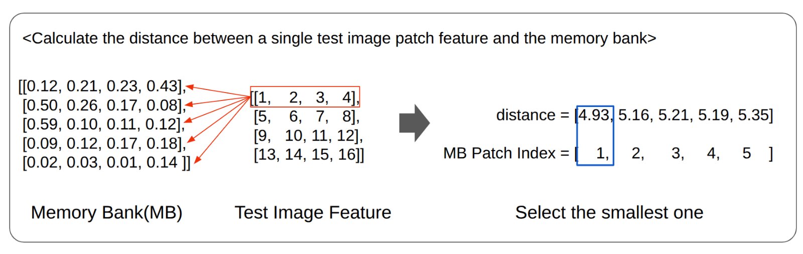
a-1. Calculate the Euclidean distances between a single test image patch and all patches in the memory bank, then select the minimum distance.
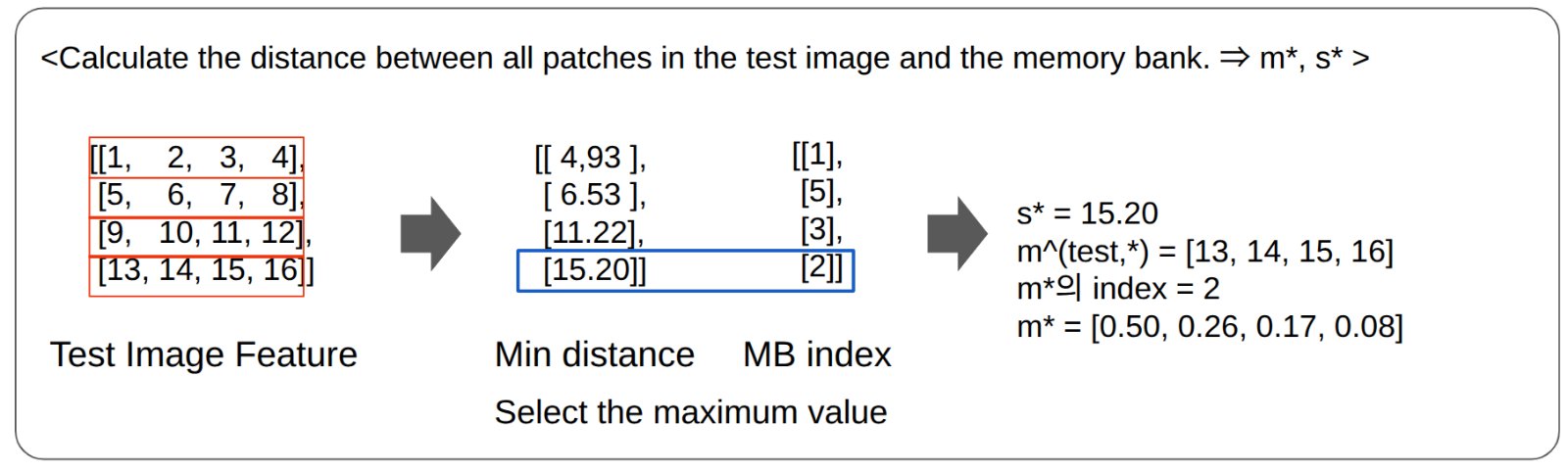
a-2. Calculate the minimum distance for all test patches, then find the patch in the memory bank associated with the maximum distance = m*
b-1. Calculate the weights to be used for the anomaly score -> using a softmax formula
b-2. After computing the Euclidean distances between m* and the memory bank, select the top-k patches with the smallest distance values as neighbor patches = Nb(m*)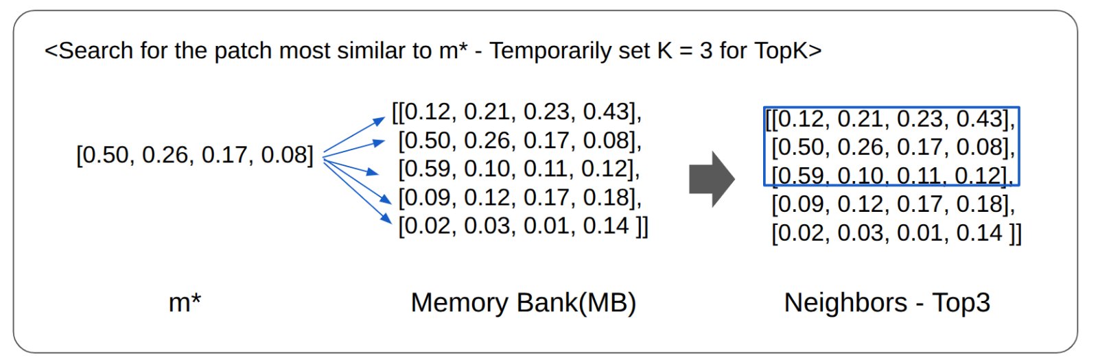
b-3. Calculate the weight
- Compute the Euclidean distances between the test patch and the neighbor patches, and use the exponentiated sum of these values as the denominator for the weight calculation.
- The numerator is calculated by taking the exponential of the minimum Euclidean distance between the test patch and the memory bank.
- The scaling weight is defined as 1 - (b-3/ b-4).
Rationale for using Softmax
- To reweight the anomaly score based on the local patch density and neighborhood context around m*.
- Large weight
- Occurs when m* is highly similar to its neighboring patches (dense nominal cluster in the memory bank).
- Indicates that the test patch distinctly deviates from a well-established normal feature cluster.
- Amplifying the weight clearly reflects a high confidence in the patch being anomalous.
- Small weight
- Occurs when m* is dissimilar to its neighboring patches (sparse/isolated region in the memory bank).
- Could happen if the test patch happens to fall into an underrepresented region due to a lack of memory bank coverage.
- Since it is ambiguous whether the high distance is noise caused by insufficient coverage or an actual subtle defect, setting a lower weight mitigates false positives.
3. Once the Anomaly Score (AS) calculation is completed for all patches, restore the score map to the original image dimensions.
- Bilinear interpolation is used to upscale the anomaly score map back to the original image size.
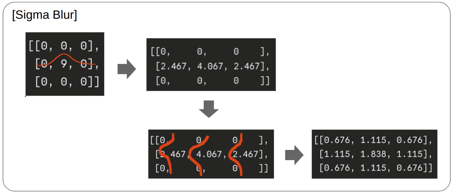
- Sigma blur (using a kernel with parameter $\sigma$) is applied to smooth the resulting heatmap.
4. Classification (Normal vs. Defective)
- Calculate the Anomaly Scores (AS) for normal samples to obtain the distribution of normal AS values. Here, the image-level AS is defined as the maximum anomaly score among all patches in an image.
- If a test image's AS falls into the 95th percentile or higher within the normal AS distribution, it is classified as an anomaly (defective).
5. Heatmap Visualization
- Trim the bottom 5% and top 5% (above the 95th percentile) from the normal AS distribution, and set the minimum and maximum of the remaining values as the reference thresholds.
- Perform min-max normalization on the restored anomaly score map (from Step 3) using these reference minimum and maximum values.
- Reason for normalization: Visualizing raw absolute values directly can cause even minor score fluctuations to look like actual defects. Normalizing relative to the normal score range ensures that only regions deviating significantly from normal bounds are highlighted and emphasized.
 GitHub
 LinkedIn